Leveraging the shape of data to improve generalization
On how to ensure that augmentations respect the shape of data.
This post serves as a quick introduction to the main concepts covered in the paper Staying on the Manifold: Geometry-Aware Noise Injection
The pros and cons of “ordinary” input noise
When assessing the usefulness of a predictive model, one critical aspect is whether it can generalize to data that was not used during training of the model. A commonly known approach to improve generalization performance is through data augmentation, where the training data set \(\mathcal{D}=\{\boldsymbol{x}_n,y_n\}_{n=1}^{N}\) is updated to contain additional, modified versions of selected training data points, e.g. \(\boldsymbol{x}_n \in \mathbb{R}^{D}\), while the associated label $y_n$ remains fixed. There exist many augmentation mechanisms but they often take structural forms, such as rotations or translations of image data. Alternatively, augmentations can be random variations of training points.
This note covers an approach based on random variations of training data, while leveraging the structure of the data points themselves. Random variations of inputs is often referred to as noise injection on the inputs, and back in 1995 Bishop
Though this approach is simple, it has a major limitation if the data is structured: we risk violating the true structure of the data when generating augmented data. We will refer to the structure of the data as the data manifold which is a lower-dimensional object in the $D$-dimensional input space $\mathbb{R}^D$, and according to the manifold hypothesis, such manifolds tend to form for high-dimensional data.
In specific cases, we might be able to characterize the manifold exactly or an approximation of it. As an example, assume that the Earth is perfectly round, in which case we can model observations on the Earth as lying on a sphere. In Figure 1 we show the effect of adding “ordinary” (meaning Gaussian) noise to a data point lying on the sphere. The augmented sample is pushed away from the manifold, making it clear that Gaussian input noise does not respect the geometry of the data.

Restricting input noise to the data manifold
Rather than adding Gaussian noise to data points, we now define geometry-aware approaches to ensure that augmented data points stay on the data manifold. We will distinguish between the input space (or ambient space) where the data manifold lives and the parameter space $\mathcal{U} \subseteq \mathbb{R}^d$ where coordinates define positions on the manifold through a parameterization $X: \mathcal{U} \rightarrow \mathbb{R}^D$ which we interchangeably refer to as the chart.
The sphere $\mathbb{S}^2$: We will consider the sphere as a running example. One way to parameterize it is by the chart:
\[X: \mathbb{R}^2 \rightarrow \mathbb{S}^2 \subset \mathbb{R}^3, \qquad X(u_1, u_2) = \begin{pmatrix} \sin u_1 \cos u_2 \\\ \sin u_1 \sin u_2 \\\ \cos u_1 \end{pmatrix}\]where $u_1 \in [0,\pi]$ and $u_2 \in [0,2\pi)$ are the angular coordinates that we collect into a single parameter space point in $\boldsymbol{u} := (u_1,u_2)$. Moving along a path $\boldsymbol{\alpha}(t)$ within the parameter space – e.g. the straight line $\boldsymbol{\alpha}(t) = (1-t) \boldsymbol{u}_A + t \boldsymbol{u}_B$ between $\boldsymbol{u}_A$ and $\boldsymbol{u}_B$ – gives a path on the manifold between the associated positions $\boldsymbol{x}_A=X(\boldsymbol{u}_A)$ and $\boldsymbol{x}_B=X(\boldsymbol{u}_B)$, when mapped through the chart, i.e. $\boldsymbol{\gamma}(t) = X(\boldsymbol{\alpha}(t))$.

Code example: defining the sphere manifold
Building on the paper’s codebase, the implementation only requires subclassing a Manifold base class and defining the parameterization $X$ as the forward call - a simplified version of the Sphere class looks as follows:
import torch
from geometric_noise.manifolds.manifold import Manifold

class Sphere(Manifold):
    def __call__(self, u):
        # u: (..., 2) tensor of parameter-space coordinates (u_1, u_2)
        u1, u2 = u[..., 0], u[..., 1]
        x = torch.stack([
            torch.sin(u1) * torch.cos(u2),
            torch.sin(u1) * torch.sin(u2),
            torch.cos(u1),
        ], dim=-1)
        return x
In principle that’s the only thing you need to write. Because $X$ has a closed form, the Jacobian $\mathbf{J}_X$ and metric $g$ derived below could be hard-coded for speed, but the Manifold base class already gives you jacobian, metric, christoffel_symbols, geodesic, and brownian_motion for free, computed via automatic differentiation straight from __call__ – so the same few lines of code work whether $X$ is a closed form or a learned function, as we will see later in the note.
Tangential noise
Locally, we can approximate the manifold by its tangent space, which is spanned by the columns of the Jacobian of $X$. The Jacobian is \(\mathbf{J}_X(\boldsymbol{u}) = \begin{bmatrix} \frac{\partial X}{\partial u_1} & \cdots & \frac{\partial X}{\partial u_d} \end{bmatrix} \in \mathbb{R}^{D \times d}\) and for our working example with the sphere, we can derive it by hand:
\[\mathbf{J}_X(u_1, u_2) = \begin{bmatrix} \frac{\partial X}{\partial u_1} & \frac{\partial X}{\partial u_2} \end{bmatrix} = \begin{bmatrix} \cos u_1 \cos u_2 & -\sin u_1 \sin u_2 \\\ \cos u_1 \sin u_2 & \sin u_1 \cos u_2 \\\ -\sin u_1 & 0 \end{bmatrix} \in \mathbb{R}^{3 \times 2}\]Exercise: derive the Jacobian of $X$
The two columns of the Jacobian are just the derivatives of $X(u_1,u_2)$ with respect to $u_1$ and $u_2$ respectively:
\[\frac{\partial X}{\partial u_1} = \begin{pmatrix}\cos u_1\cos u_2\\ \cos u_1\sin u_2\\ -\sin u_1\end{pmatrix}, \qquad \frac{\partial X}{\partial u_2} = \begin{pmatrix}-\sin u_1\sin u_2\\ \sin u_1\cos u_2\\ 0\end{pmatrix}.\]Stacking these two vectors side by side as columns gives $\mathbf{J}_X(u_1,u_2)$ above.
In code, you do not need to do this by hand – jacobian on the Manifold base class computes exactly this via automatic differentiation:
manifold = Sphere()
u = torch.tensor([[1.0, 0.5]])  # a single (u_1, u_2) point
J = manifold.jacobian(u)  # shape (B, D, d) = (1, 3, 2)
A simple geometry-aware noise injection method is to pull ambient space noise samples closer to the manifold by projecting $\boldsymbol{\epsilon}$ onto the tangent space, which removes whatever part of the injected noise that points off the manifold. The tangential noise sample is then simply $\boldsymbol{\epsilon}_\top = \mathbf{P}\boldsymbol{\epsilon}$ where $\mathbf{P}$ is the projection matrix for the base point. We refer to the paper for further details and note that tangential noise is still not exactly on the manifold as the tangent space only intersects with the manifold at the base point $\boldsymbol{x}=X(\boldsymbol{u})$.

Code example: projecting noise onto the tangent space
The Manifold base class builds the projection matrix from the Jacobian – it takes the cross product of the two Jacobian columns to get the (single) normal direction, then projects out that direction.
For an example point $(u_1,u_2)=(1.0, 0.5)$ with a concrete noise vector, obtaining the tangent space sample is straight forward:
u = torch.tensor([[1.0, 0.5]])
manifold = Sphere()

J = manifold.jacobian(u)[0]                 # J_X(u_1,u_2), shape (3, 2)
P = manifold.tangent_projection_matrix(J)   # projection matrix, shape (3, 3)

eps = torch.tensor([0.4, -0.3, 0.7])        # a concrete ambient noise sample
eps_top = P @ eps                           # projected onto the tangent space
Note that $\boldsymbol{\epsilon}$ had a component sticking straight out of the sphere (along $\boldsymbol{x}$), while $\boldsymbol{\epsilon}_\top$ does not. You can check that $\boldsymbol{\epsilon}_\top \cdot \boldsymbol{x} \approx 0$ up to floating-point error, confirming it really does lie flat in the tangent plane at $\boldsymbol{x}$.
Geodesic noise
A geodesic can conceptually be thought of as the straightest path on the manifold. In the parameter space, this is generally different from the straight line shown earlier since manifolds are often curved objects – this is what bends the motion of a geodesic. In comparison to tangent space noise, adding noise via geodesics means that the augmented samples stay on the manifold by construction.
We refer the interested reader to the paper for a proper definition of geodesics but note that geodesics rely on a metric. Loosely speaking, a metric $g$ tells you how to measure lengths and angles on the data manifold using only the parameter-space coordinates: a small step $d\boldsymbol{u}$ from $\boldsymbol{u}$ approximately corresponds to a step $\mathbf{J}_X(\boldsymbol{u})\, d\boldsymbol{u}$ on the manifold. Its squared length defines the inner product on the manifold:
\[d \boldsymbol{u}^\top \mathbf{J}_X(\boldsymbol{u})^\top \mathbf{J}_X(\boldsymbol{u}) d \boldsymbol{u} = d \boldsymbol{u}^\top g(\boldsymbol{u}) d \boldsymbol{u}\]where $g(\boldsymbol{u})$ is the metric. For the example with the sphere, the metric induced by $X$ is:
\[g(u_1, u_2) = \begin{bmatrix} 1 & 0 \\\ 0 & \sin^2 u_1 \end{bmatrix}\]Intuitively, the two diagonal entries of $g$ measure how far a step in the parameter space actually gets you on the sphere. Figure 4 visualizes this with the indicatrix of the metric at each point: the ellipse you get by mapping a small unit circle of parameter-space directions onto the sphere through $X$. A step along $u_1$ always covers the same distance, no matter where you are – this is the $1$ in $g$. A step along $u_2$, on the other hand, moves you sideways around a circle of latitude, and since those circles shrink to a point at the poles where \(u_1 \in \{0,\pi\}\), the same-sized step covers less and less distance the closer you get to a pole – this is the $\sin^2 u_1$ term. That is why the indicatrices in Figure 4 stay the same height everywhere but grow narrower near the top and bottom.

A geodesic can be computed by solving an initial value problem (IVP) posed by the geodesic equations. In essence, this requires defining the initial position of the path $\boldsymbol{u}_0=X^{-1}(\boldsymbol{x}_0)$ and the initial velocity $\boldsymbol{v}_0$ that determines the direction to move.

Code example: the geodesic equation
A curve $\boldsymbol{\alpha}(t)$ in parameter space maps to a geodesic on the manifold if and only if it satisfies, for every coordinate $k$,
\[\ddot{\alpha}_k(t) = -\sum_{i,j} \dot{\alpha}_i(t)\dot{\alpha}_j(t)\, \Gamma^k_{ij}(\boldsymbol{\alpha}(t)),\]where the $\Gamma^k_{ij}$ are the Christoffel symbols. These are correction terms computed from the metric $g$ that capture how the manifold curves. We skip the somewhat technical derivation of the $\Gamma^k_{ij}$ here and refer to the paper for further details and a worked-out example.
In code, christoffel_symbols computes the $\Gamma^k_{ij}$ (again via automatic differentiation from metric), and geodesic uses them to solve the IVP for you:
position = torch.tensor([1.0, 0.5])   # starting point (u_1, u_2)
velocity = torch.tensor([0.1, -0.2])  # initial velocity
ambient_curve, param_curve = manifold.geodesic(position, init_v=velocity)
Brownian motion noise
Rather than doing a geodesic step, a final augmentation strategy is that of doing a random walk on the manifold. One approach to this is a Brownian motion, where we sequentially do minor random perturbations of the data, while respecting the geometry. In flat space this is written as a stochastic differential equation (SDE) on the form $dx(t) = dB(t)$, where $dB(t)$ is an infinitesimal Gaussian increment – simulating it just means repeatedly adding a small amount of Gaussian noise, over and over. To restrict this random walk to the manifold, we define the same idea directly in the parameter space, but the noise now has to be reshaped by the metric $g$ so that it respects the manifold’s geometry.

Code example: Brownian motion on a manifold
Naively adding flat Gaussian noise at every step, as above, would drift off the manifold just like ambient noise does. Instead, we define a Brownian motion in the parameter space of a Riemannian manifold with metric $g$ as follows
The noise term is the same Gaussian increment $dB(t)$ introduced earlier, just passed through $\sqrt{g^{-1}}$ so that a step of a given size always corresponds to the same physical distance on the manifold. The drift term is a correction accounting for how $g$ itself changes across the manifold, so the random walk does not end up systematically biased toward one region. We refer the interested reader to the paper and related works for further details.
In code, brownian_motion discretizes this SDE and computes an instance of it as follows:
position = torch.tensor([1.0, 0.5])  # starting point (u_1, u_2)
ambient_traj, param_traj = manifold.brownian_motion(
  position,
  diffusion_time=0.1,
  num_steps=100
)
What if I do not know the shape of my data?
If you do not know the shape of your data, do not give up just yet. Why? Because we can approximate the data manifold using advanced machine learning techniques such as generative models or autoencoders
An autoencoder consists of an encoder $f_e: \mathbb{R}^D \rightarrow \mathbb{R}^d$ and a decoder $f_d: \mathbb{R}^d \rightarrow \mathbb{R}^D$, both parameterized by weights $\boldsymbol{\theta} \in \Theta$ that we fit by minimizing the reconstruction error:
\[\arg \min_{\boldsymbol{\theta}} \frac{1}{N} \sum_{n=1}^N (\boldsymbol{x}_n - f_d(f_e(\boldsymbol{x}_n)))^2\]Once trained, the decoder $f_d$ itself plays the role of the chart $X$ from before, and the parameter space coordinate is instead the latent code $\boldsymbol{z} = f_e(\boldsymbol{x}) \in \mathcal{Z} \subseteq \mathbb{R}^d$, so that a reconstruction is given by $\tilde{\boldsymbol{x}} = f_d(\boldsymbol{z})$. Remark our use of the term parameter space, since the weight space $\Theta$ would often be referred to as the parameter space of the autoencoder, however we use it to describe the parameter space of the learned data manifold $\mathcal{Z}$.
For a learned data manifold with the chart $X:=f_e(\cdot)$ and approximate inverse $X^{-1}:=f_d(\cdot)$, we do not need further adjustments to define the three geometry-aware noise injection strategies considered previously: all we need is the Jacobian of the decoder \(\mathbf{J}_{f_d}(\boldsymbol{z})\) which gives \(g_{f_d}(\boldsymbol{z}) = \mathbf{J}_{f_d}(\boldsymbol{z})^\top \mathbf{J}_{f_d}(\boldsymbol{z})\). Though the metric does not have a closed form when $f_d$ is parameterized by a neural network, we can efficiently evaluate it using automatic differentiation.
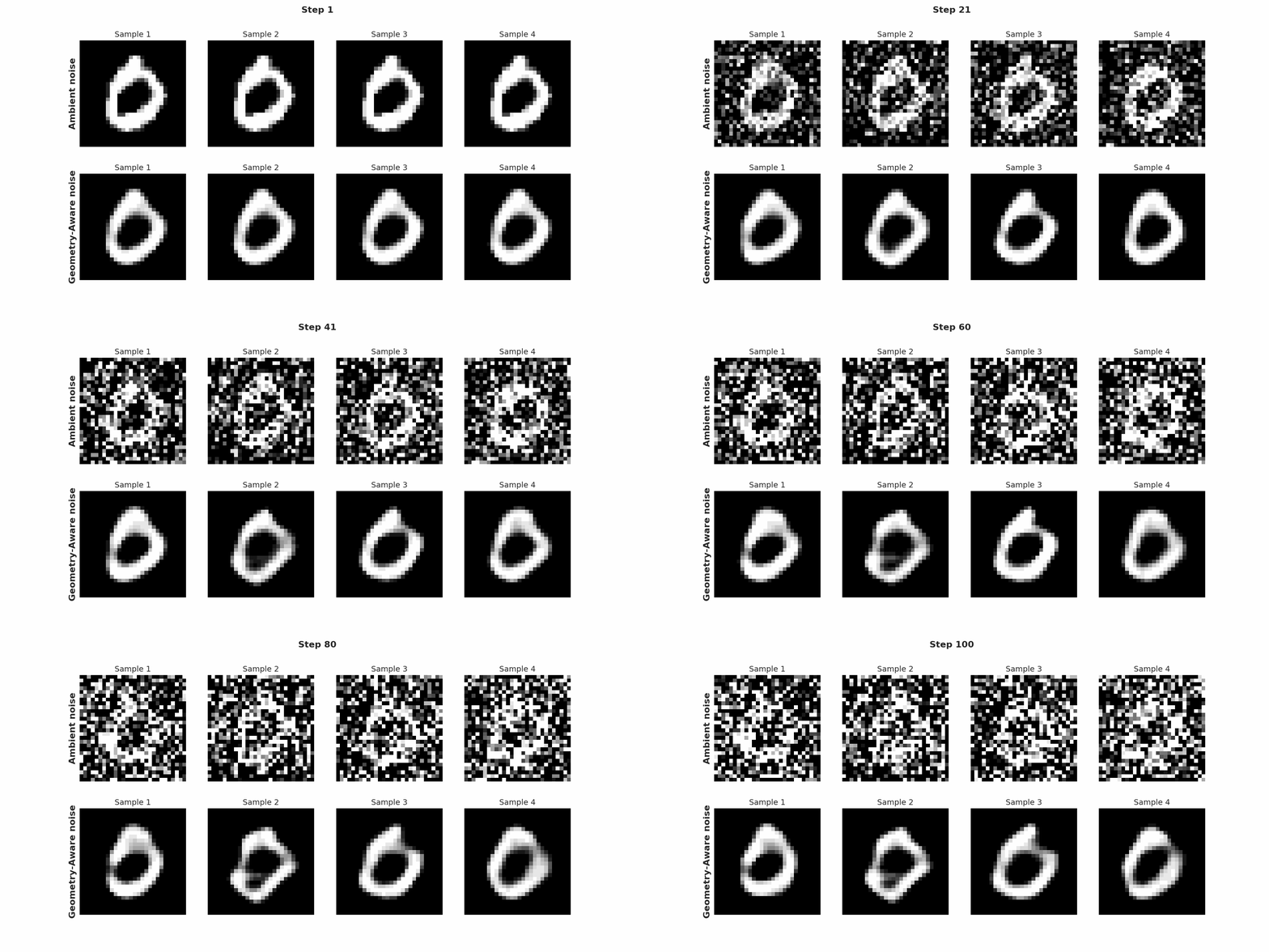
As an example, we train an autoencoder and run four different Brownian motions from the exact same input sample of the digit “0”. In addition we also consider Brownian motion in the ambient space, which at time $T$ corresponds to adding Gaussian noise with spread $\sqrt{T}$ to the input, i.e. the original approach considered by Bishop. The effect is clear: even though the parameterization only approximates the data manifold, the geometry-aware perturbations are visually meaningful perturbations of the original input digit. In contrast, ambient Brownian motion destroys the input signal as time increases.
But does it improve generalization?
Yes indeed, and we also have theory on this! You can find results in the full paper.
If you want to try it out yourself, we provide the example code for MNIST in an associated notebook. Future research directions could consider more advanced approximations of the data manifold, e.g. using generative models.